Abstract¶

In September 2021, a significant jump in seismic activity on the island of La Palma (Canary Islands, Spain) signaled the start of a volcanic crisis that still continues at the time of writing. Earthquake data is continually collected and published by the Instituto Geográphico Nacional (IGN). We have created an accessible dataset from this and completed preliminary data analysis which shows seismicity originating at two distinct depths, consistent with the model of a two reservoir system feeding the currently very active volcano.

Key Points¶

You may specify 1 to 3 keypoints for this PDF template

These keypoints are complete sentences and less than or equal to 140 characters

They are specific to this PDF template, so they will not appear in other exports

Keywords:La PalmaEarthquakes¶

Introduction¶

The content of your notebook may be broken into any number of markdown or code cells. Markdown cells use MyST markdown and support standard markdown typography and many directives and roles for figures, tables, equations, etc.

La Palma is one of the west most islands in the Volcanic Archipelago of the Canary Islands, a Spanish territory situated is the Atlantic Ocean where at their closest point are 100km from the African coast Figure 1 The island is one of the youngest, remains active and is still in the island forming stage.

Figures may be added to your notebook using the figure directive. They may refer to images saved in your images/ folder, images from the web, or notebook cell outputs referenced by label. The :name: is used to reference the figure in your text; a reference to the following figure is found in the paragraph above. The figure caption is given as the body of this directive.

Figure 1:Map of La Palma in the Canary Islands. Image credit NordNordWest

La Palma has been constructed by various phases of volcanism, the most recent and currently active being the Cumbre Vieja volcano, a north-south volcanic ridge that constitutes the southern half of the island.

Eruption History¶

A number of eruptions were recorded since the colonization of the islands by Europeans in the late 1400s, these are summarized in Table 1.

Simple tables may be created using the list-table directive. Similar to figures, tables may be referenced in the text by their name. The caption for this table is the first line of the directive.

Table 1:Recent historic eruptions on La Palma

Name	Year
Current	2021
Teneguía	1971
Nambroque	1949
El Charco	1712
Volcán San Antonio	1677
Volcán San Martin	1646
Tajuya near El Paso	1585
Montaña Quemada	1492

This equates to an eruption on average every 79 years up until the 1971 event. The probability of a future eruption can be modeled by a Poisson distribution (1).

Numbered equations may be defined using the math directive or in line. Equations defined with the math directive may be reference in the text by label.

p(x)=\frac{e^{-\lambda} \lambda^{x}}{x !}

(1)

Where λ is the number of eruptions per year, $\lambda=\frac{1}{79}$ in this case. The probability of a future eruption in the next $t$ years can be calculated by:

p_e = 1-\mathrm{e}^{-t \lambda}

(2)

So following the 1971 eruption the probability of an eruption in the following 50 years — the period ending this year — was 0.469. After the event, the number of eruptions per year moves to $\lambda=\frac{1}{75}$ and the probability of a further eruption within the next 50 years (2022-2071) rises to 0.487 and in the next 100 years, this rises again to 0.736.

Magma Reservoirs¶

You may add citations two ways. First, you may simply insert a markdown link to a DOI like so: Thompson et al. (1994). No additional bibliographic information is required for this approach; the reference will be looked up by DOI and added implicitly to the references. Alternatively, you may provide the bibliography directly as references.bib BibTeX file, then embed the citation by BibTeX key in your text using the @cite2023 or [@cite2023; @cite2023b] for narrative or parenthetical citations, respectively. The following paragraph provides an example of this. A single paper may combine both DOI and BibTeX citations.

Studies of the magma systems feeding the volcano, such as Marrero et al. (2019) has proposed that there are two main magma reservoirs feeding the Cumbre Vieja volcano; one in the mantle (30-40km depth) which charges and in turn feeds a shallower crustal reservoir (10-20km depth).

Figure 2:Proposed model from Marrero et al

In this paper, we look at recent seismicity data to see if we can see evidence of such a system action, see Figure 2.

Dataset¶

All data used in the notebook should be present in the data/ folder so notebooks may be executed in place with no additional input.

The earthquake dataset used in our analysis was generated from the IGN web portal this is public data released under a permissive license. Data recorded using the network of Seismic Monitoring Stations on the island. A web scraping script was developed to pull data into a machine-readable form for analysis. That code tool is available on GitHub along with a copy of recently updated data.

Main Timeline Figure¶

Code cells may be seamlessly interleaved with markdown cells. Currently, with a single-article submission, code cannot be hidden in the output document.

import pandas as pd
import matplotlib
import matplotlib.pyplot as plt
%matplotlib inline
import seaborn as sns
import numpy as np
sns.set_theme(style="whitegrid")

def make_category_columns(df):
    df['Depth'] = 'Shallow (<18km)'
    df.loc[(df['Depth(km)'] >= 18) & (df['Depth(km)'] <= 28), 'Depth'] = 'Interchange (18km>x>28km)'
    df.loc[df['Depth(km)'] >= 28, 'Depth'] = 'Deep (>28km)'

    df['Mag'] = 0
    df.loc[(df['Magnitude'] >= 1) & (df['Magnitude'] <= 2), 'Mag'] = 1
    df.loc[(df['Magnitude'] >= 2) & (df['Magnitude'] <= 3), 'Mag'] = 2
    df.loc[(df['Magnitude'] >= 3) & (df['Magnitude'] <= 4), 'Mag'] = 3
    df.loc[(df['Magnitude'] >= 4) & (df['Magnitude'] <= 5), 'Mag'] = 4

    return df

Visualising Long term earthquake data¶

Data taken directly from the IGN Catalog

Supported cell outputs below include pandas dataframe, raw text output, matplotlib plot, and seaborn plot.

df_ign = pd.read_csv('./data/lapalma_ign.csv')
df_ign = make_category_columns(df_ign)
df_ign.head()

df_ign['DateTime'] = pd.to_datetime(df_ign['Date'] + ' ' + df_ign['Time'])
df_ign['DateTime'];

df_ign_early = df_ign[df_ign['DateTime'] < '2021-09-11']
df_ign_pre = df_ign[(df_ign['DateTime'] >= '2021-09-11')&(df_ign['DateTime'] < '2021-09-19 14:13:00')]
df_ign_phase1 = df_ign[(df_ign['DateTime'] >= '2021-09-19 14:13:00')&(df_ign['DateTime'] < '2021-10-01')]
df_ign_phase2 = df_ign[(df_ign['DateTime'] >= '2021-10-01')&(df_ign['DateTime'] < '2021-12-01')]
df_ign_phase3 = df_ign[(df_ign['DateTime'] >= '2021-12-01')&(df_ign['DateTime'] <= '2021-12-31')]

df_erupt = df_ign[(df_ign['Date'] < '2022-01-01') & (df_ign['Date'] > '2021-09-11')]

df_erupt_1 = df_erupt[df_erupt['Magnitude'] < 1.0]
df_erupt_2 = df_erupt[(df_erupt['Magnitude'] >= 1.0)&(df_erupt['Magnitude'] < 2.0)]
df_erupt_3 = df_erupt[(df_erupt['Magnitude'] >= 2.0)&(df_erupt['Magnitude'] < 3.0)]
df_erupt_4 = df_erupt[(df_erupt['Magnitude'] >= 3.0)&(df_erupt['Magnitude'] < 4.0)]
df_erupt_5 = df_erupt[df_erupt['Magnitude'] > 4.0]

tab20_colors = (
    (0.12156862745098039, 0.4666666666666667,  0.7058823529411765  ),  # 1f77b4
    (0.6823529411764706,  0.7803921568627451,  0.9098039215686274  ),  # aec7e8
    (1.0,                 0.4980392156862745,  0.054901960784313725),  # ff7f0e
    (1.0,                 0.7333333333333333,  0.47058823529411764 ),  # ffbb78
    (0.17254901960784313, 0.6274509803921569,  0.17254901960784313 ),  # 2ca02c
    (0.596078431372549,   0.8745098039215686,  0.5411764705882353  ),  # 98df8a
    (0.8392156862745098,  0.15294117647058825, 0.1568627450980392  ),  # d62728
    (1.0,                 0.596078431372549,   0.5882352941176471  ),  # ff9896
    (0.5803921568627451,  0.403921568627451,   0.7411764705882353  ),  # 9467bd
    (0.7725490196078432,  0.6901960784313725,  0.8352941176470589  ),  # c5b0d5
    (0.5490196078431373,  0.33725490196078434, 0.29411764705882354 ),  # 8c564b
    (0.7686274509803922,  0.611764705882353,   0.5803921568627451  ),  # c49c94
    (0.8901960784313725,  0.4666666666666667,  0.7607843137254902  ),  # e377c2
    (0.9686274509803922,  0.7137254901960784,  0.8235294117647058  ),  # f7b6d2
    (0.4980392156862745,  0.4980392156862745,  0.4980392156862745  ),  # 7f7f7f
    (0.7803921568627451,  0.7803921568627451,  0.7803921568627451  ),  # c7c7c7
    (0.7372549019607844,  0.7411764705882353,  0.13333333333333333 ),  # bcbd22
    (0.8588235294117647,  0.8588235294117647,  0.5529411764705883  ),  # dbdb8d
    (0.09019607843137255, 0.7450980392156863,  0.8117647058823529  ),  # 17becf
    (0.6196078431372549,  0.8549019607843137,  0.8980392156862745),    # 9edae5
)

from matplotlib.patches import Rectangle

import datetime as dt
from matplotlib.dates import date2num, num2date

matplotlib.rcParams['font.family'] = "sans-serif"
matplotlib.rcParams['xtick.labelsize'] = 14
matplotlib.rcParams['ytick.labelsize'] = 14
matplotlib.rcParams['ytick.labelleft'] = True
matplotlib.rcParams['ytick.labelright'] = True

%matplotlib inline
fig = matplotlib.pyplot.figure(figsize=(24,12))
fig.tight_layout()
# Creating axis
# add_axes([xmin,ymin,dx,dy])
ax_min = fig.add_axes([0.01, 0.01, 0.01, 0.01])
ax_min.axis('off')
ax_max = fig.add_axes([0.99, 0.99, 0.01, 0.01])
ax_max.axis('off')

ax_timeline = fig.add_axes([0.04, 0.1, 0.92, 0.85])
ax_timeline.spines["top"].set_visible(False)
ax_timeline.spines["right"].set_visible(False)
ax_timeline.spines["left"].set_visible(False)
ax_timeline.grid(axis='x')


ax_timeline.axvline(x=dt.datetime(2021, 9, 19, 14, 13), ymin=0.075, ymax=0.98, color='r', linewidth=3)


def make_scatter(df, c, alpha=0.8):
    M = 3*np.exp2(1.3*df['Magnitude'])
    return ax_timeline.scatter(df['DateTime'], df['Depth(km)'], s=M, c=c, alpha=alpha, edgecolor='black', linewidth=0.5, zorder=2);

# make_scatter(df_erupt, c=tab20c_colors[-1])
points_1 = make_scatter(df_erupt_1, c=[tab20_colors[12]], alpha=0.3)
points_2 = make_scatter(df_erupt_2, c=[tab20_colors[16]], alpha=0.4)
points_3 = make_scatter(df_erupt_3, c=[tab20_colors[4]], alpha=0.5)
points_4 = make_scatter(df_erupt_4, c=[tab20_colors[2]], alpha=0.6)
points_5 = make_scatter(df_erupt_5, c=[tab20_colors[6]], alpha=0.8)

ax_timeline.tick_params(axis='x', labelrotation=0, bottom=True)
ax_timeline.set_ylabel('')
ax_timeline.yaxis.set_ticks_position('both')
ax_timeline.yaxis.set_ticks_position('both')

xticks = ax_timeline.get_xticks()
new_xticks = [date2num(pd.to_datetime('2021-09-11')),
    date2num(pd.to_datetime('2021-09-19 14:13:00'))]
new_xticks = np.append(new_xticks, xticks[2:-1])
ax_timeline.set_xticks(new_xticks)

ax_timeline.invert_yaxis()
ax_timeline.spines['bottom'].set_position(('data', 45))
ax_timeline.margins(tight=True, x=0)
ax_timeline.legend(
    [points_1, points_2, points_3, points_4, points_5],
    ['0 < M <= 1','1 < M <= 2','2 < M <= 3','3 < M <= 4','M > 4'],
    loc='lower left', bbox_to_anchor=(0.01, 0.1, 0.15, 0.1), fancybox=True,
    borderpad=1.0, labelspacing=1, mode="expand", title="Event Magnitude (M)",
    fontsize=14, title_fontsize=14, framealpha=1)

ax_timeline.set_ylim(ax_timeline.get_ylim()[0], -9)

plt.annotate('ERUPTION', (0.055, 0.42), rotation=90, xycoords='axes fraction', fontweight='bold', fontsize=20, color='r')
plt.annotate('Pre\nEruptive\nSwarm', (0.035, 0.88), rotation=0, xycoords='axes fraction', fontweight='bold', fontsize=20, color='b', horizontalalignment='center')
plt.annotate('Early Eruptive\nPhase', (0.12, 0.9), rotation=0, xycoords='axes fraction', fontweight='bold', fontsize=20, color='orange', horizontalalignment='center')
plt.annotate('Main Eruptive Phase\n(sustained gas and lava ejection)', (0.45, 0.9), rotation=0, xycoords='axes fraction', fontweight='bold', fontsize=20, color='green', horizontalalignment='center')
plt.annotate('Final Eruptive Phase\n(reducing gas and lava ejection)', (0.86, 0.9), rotation=0, xycoords='axes fraction', fontweight='bold', fontsize=20, color='r', horizontalalignment='center')

ax_timeline.add_patch(Rectangle((date2num(pd.to_datetime('2021-09-11')), -8), date2num(pd.to_datetime('2021-09-19 14:13:00'))-date2num(pd.to_datetime('2021-09-11')), 53, color=tab20_colors[0], zorder=1, alpha=0.1))
ax_timeline.add_patch(Rectangle((date2num(pd.to_datetime('2021-09-19 14:13:00')), -8), date2num(pd.to_datetime('2021-10-01'))-date2num(pd.to_datetime('2021-09-19 14:13:00')), 53, color=tab20_colors[2], zorder=1, alpha=0.1))
ax_timeline.add_patch(Rectangle((date2num(pd.to_datetime('2021-10-01')), -8), date2num(pd.to_datetime('2021-12-01'))-date2num(pd.to_datetime('2021-10-01')), 53, color=tab20_colors[4], zorder=1, alpha=0.1))
ax_timeline.add_patch(Rectangle((date2num(pd.to_datetime('2021-12-01')), -8), date2num(pd.to_datetime('2021-12-31'))-date2num(pd.to_datetime('2021-12-01'))+1, 53, color=tab20_colors[6], zorder=1, alpha=0.1));

ax_timeline.set_title("Recorded seismicity during the La Palma eruption 11 September - 15 December 2021 (INVOLCAN Dataset)", dict(fontsize=24), pad=20)
ax_timeline.set_ylabel("Depth (km)", dict(fontsize=20), labelpad=20)
ax_timeline.set_xlabel("Eruption Timeline", dict(fontsize=20), labelpad=20);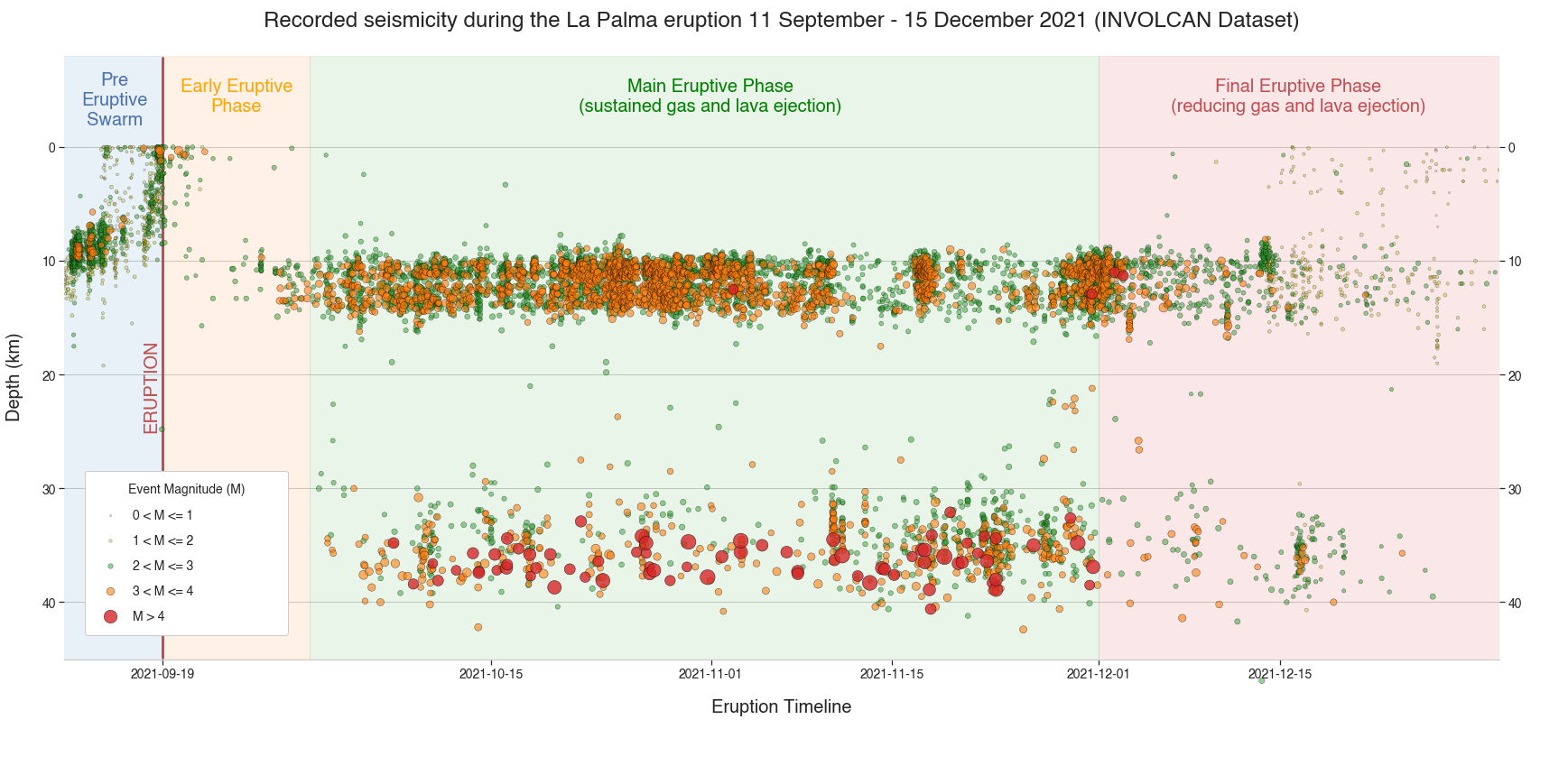

Cumulative Distrubtion Plots¶

def cumulative_events_mag_depth(df, hue='Depth', kind='scatter', ax=None, dpi=100, palette=None, kde=True):
    matplotlib.rcParams['ytick.labelright'] = False
    g = sns.jointplot(x="Magnitude", y="Depth(km)", data=df,
                      kind=kind, hue=hue, height=10, space=0.1, marginal_ticks=False, ratio=8, alpha=0.6,
                      hue_order=['Shallow (<18km)', 'Interchange (18km>x>28km)', 'Deep (>28km)'],
                      ax=ax, palette=palette, ylim=(-2,50), xlim=(0.3,5.6), edgecolor=".2", marginal_kws=dict(bins=20, hist_kws={'edgecolor': 'black'}))
    if kde:
        g.plot_joint(sns.kdeplot, color="b", zorder=1, levels=15, ax=ax)
    g.fig.axes[0].invert_yaxis();
    g.fig.set_dpi(dpi)

import warnings

with warnings.catch_warnings():
    warnings.simplefilter("ignore")
    cumulative_events_mag_depth(df_ign, hue=None, dpi=200)
    plt.suptitle('Cumulative Events 01-01-2017 to 01-01-2022', y=1.01);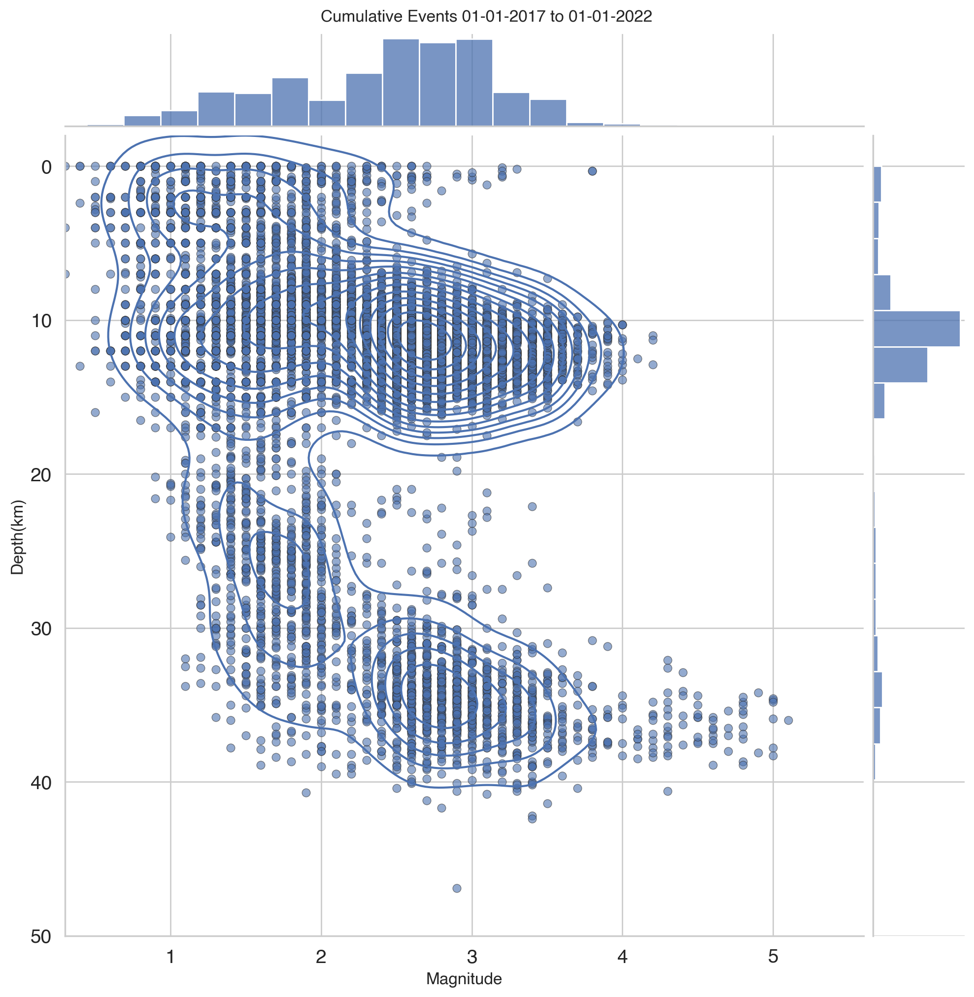

Results¶

The dataset was loaded into this Jupyter notebook and filtered down to La Palma events only. This results in 5465 data points which we then visualized to understand their distributions spatially, by depth, by magnitude and in time.

From our analysis above, we can see 3 different systems in play.

Firstly, the shallow earthquake swarm leading up to the eruption on 19th September, related to significant surface deformation and shallow magma intrusion.

After the eruption, continuous shallow seismicity started at 10-15km corresponding to magma movement in the crustal reservoir.

Subsequently, high magnitude events begin occurring at 30-40km depths corresponding to changes in the mantle reservoir. These are also continuous but occur with a lower frequency than in the crustal reservoir.

Conclusions¶

From the analysis of the earthquake data collected and published by IGN for the period of 11 September through to 9 November 2021. Visualization of the earthquake events at different depths appears to confirm the presence of both mantle and crustal reservoirs as proposed by Marrero et al. (2019).

Data Availability¶

A web scraping script was developed to pull data into a machine-readable form for analysis. That code tool is available on GitHub along with a copy of recently updated data.

References¶

Thompson, J. D., Higgins, D. G., & Gibson, T. J. (1994). CLUSTAL W: improving the sensitivity of progressive multiple sequence alignment through sequence weighting, position-specific gap penalties and weight matrix choice. Nucleic Acids Research, 22(22), 4673–4680. 10.1093/nar/22.22.4673
Marrero, J., García, A., Berrocoso, M., Llinares, Á., Rodríguez-Losada, A., & Ortiz, R. (2019). Strategies for the development of volcanic hazard maps in monogenetic volcanic fields: the example of La Palma (Canary Islands). Journal of Applied Volcanology, 8. 10.1186/s13617-019-0085-5