La Palma Earthquakes

Introduction

La Palma is one of the west most islands in the Volcanic Archipelago of the Canary Islands, a Spanish territory situated is the Atlantic Ocean where at their closest point are 100km from the African coast Figure 1. The island is one of the youngest, remains active and is still in the island forming stage.

Figure 1: Map of La Palma in the Canary Islands. Image credit NordNordWest

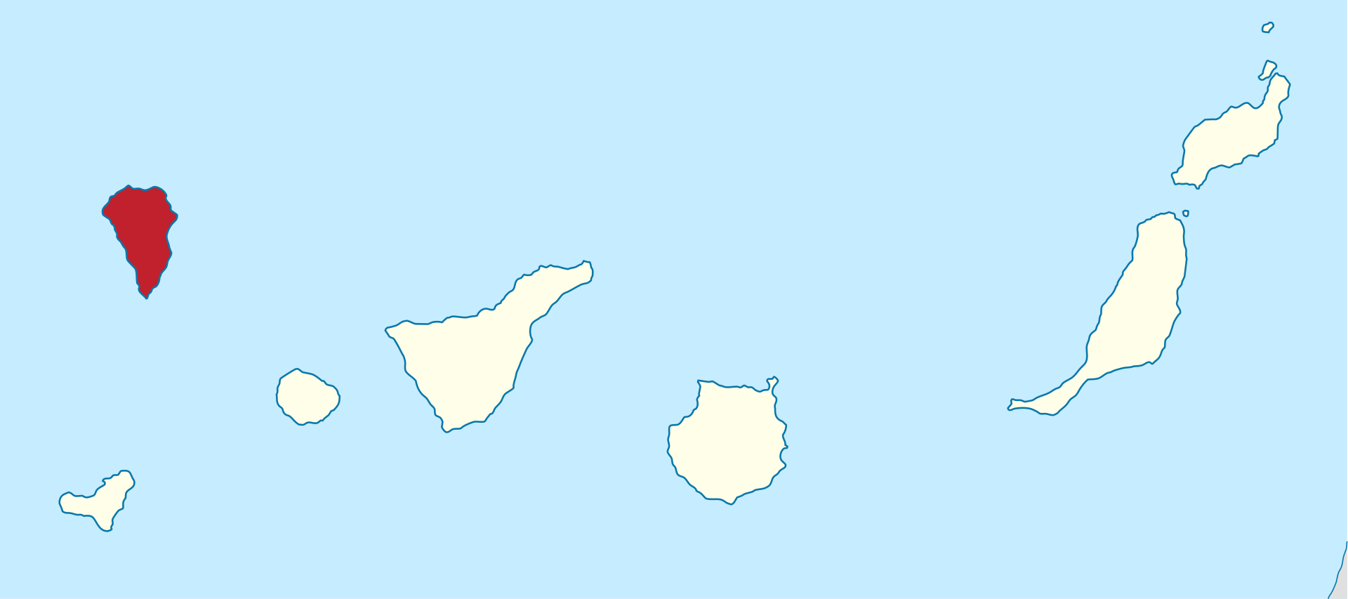
La Palma has been constructed by various phases of volcanism, the most recent and currently active being the Cumbre Vieja volcano, a north-south volcanic ridge that constitutes the southern half of the island.

Eruption History

A number of eruptions were recorded since the colonization of the islands by Europeans in the late 1400s, these are summarised in Table 1.

Table 1: Recent historic eruptions on La Palma

Name	Year
Current	2021
Teneguía	1971
Nambroque	1949
El Charco	1712
Volcán San Antonio	1677
Volcán San Martin	1646
Tajuya near El Paso	1585
Montaña Quemada	1492

This equates to an eruption on average every 79 years up until the 1971 event. The probability of a future eruption can be modeled by a Poisson distribution Equation 1.

\[ p(x)=\frac{e^{-\lambda} \lambda^{x}}{x !} \tag{1}\]

Where \(\lambda\) is the number of eruptions per year, \(\lambda=\frac{1}{79}\) in this case. The probability of a future eruption in the next \(t\) years can be calculated by:

\[ p_e = 1-\mathrm{e}^{-t \lambda} \tag{2}\]

So following the 1971 eruption the probability of an eruption in the following 50 years — the period ending this year — was 0.469. After the event, the number of eruptions per year moves to \(\lambda=\frac{1}{75}\) and the probability of a further eruption within the next 50 years (2022-2071) rises to 0.487 and in the next 100 years, this rises again to 0.736.

Magma Reservoirs

Studies of the magma systems feeding the volcano, such as Marrero et al. (2019) has proposed that there are two main magma reservoirs feeding the Cumbre Vieja volcano; one in the mantle (30-40km depth) which charges and in turn feeds a shallower crustal reservoir (10-20km depth).

Figure 2: Proposed model from Marrero et al

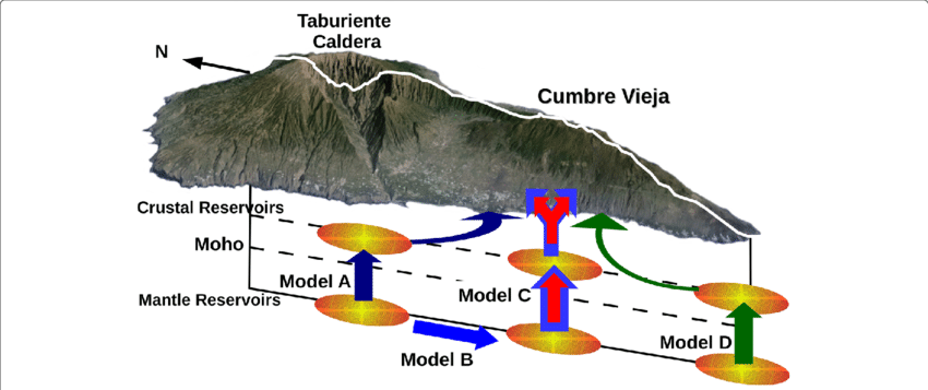
In this paper, we look at recent seismicity data to see if we can see evidence of such a system action, see Figure 2.

Dataset

The earthquake dataset used in our analysis was generated from the IGN web portal this is public data released under a permissive license. Data recorded using the network of Seismic Monitoring Stations on the island. A web scraping script was developed to pull data into a machine-readable form for analysis. That code tool is available on GitHub along with a copy of recently updated data.

Main Timeline Figure

In [1]:

import pandas as pd
import matplotlib
import matplotlib.pyplot as plt
%matplotlib inline
import seaborn as sns
import numpy as np
sns.set_theme(style="whitegrid")

In [2]:

def make_category_columns(df):
    df['Depth'] = 'Shallow (<18km)'
    df.loc[(df['Depth(km)'] >= 18) & (df['Depth(km)'] <= 28), 'Depth'] = 'Interchange (18km>x>28km)'
    df.loc[df['Depth(km)'] >= 28, 'Depth'] = 'Deep (>28km)'
    
    df['Mag'] = 0
    df.loc[(df['Magnitude'] >= 1) & (df['Magnitude'] <= 2), 'Mag'] = 1
    df.loc[(df['Magnitude'] >= 2) & (df['Magnitude'] <= 3), 'Mag'] = 2
    df.loc[(df['Magnitude'] >= 3) & (df['Magnitude'] <= 4), 'Mag'] = 3
    df.loc[(df['Magnitude'] >= 4) & (df['Magnitude'] <= 5), 'Mag'] = 4    
    
    return df

Visualising Long term earthquake data

Data taken directly from the IGN Catalog

In [3]:

df_ign = pd.read_csv('./data/lapalma_ign.csv')
df_ign = make_category_columns(df_ign)
df_ign.head()

	Event	Date	Time	Latitude	Longitude	Depth(km)	Intensity	Magnitude	Type Mag	Location	DateTime	Timestamp	Swarm	Phase	Depth	Mag
0	es2017eugju	2017-03-09	23:44:06	28.5346	-17.8349	26.0		1.6	4	NE FUENCALIENTE DE LA PALMA.IL	2017-03-09 23:44:06	1489103046000000000	0.0	0	Interchange (18km>x>28km)	1
1	es2017euhlh	2017-03-10	00:16:10	28.5491	-17.8459	27.0		2.0	4	N FUENCALIENTE DE LA PALMA.ILP	2017-03-10 00:16:10	1489104970000000000	0.0	0	Interchange (18km>x>28km)	2
2	es2017cpaoh	2017-03-10	00:16:11	28.5008	-17.8863	20.0		2.1	4	W LOS CANARIOS.ILP	2017-03-10 00:16:11	1489104971000000000	0.0	0	Interchange (18km>x>28km)	2
3	es2017eunnk	2017-03-10	03:20:26	28.5204	-17.8657	30.0		1.6	4	NW FUENCALIENTE DE LA PALMA.IL	2017-03-10 03:20:26	1489116026000000000	0.0	0	Deep (>28km)	1
4	es2017kajei	2017-08-21	02:06:55	28.5985	-17.7156	0.0		1.6	4	E EL PUEBLO.ILP	2017-08-21 02:06:55	1503281215000000000	0.0	0	Shallow (<18km)	1

In [4]:

df_ign['DateTime'] = pd.to_datetime(df_ign['Date'] + ' ' + df_ign['Time'])
df_ign['DateTime'];

In [5]:

df_ign_early = df_ign[df_ign['DateTime'] < '2021-09-11']
df_ign_pre = df_ign[(df_ign['DateTime'] >= '2021-09-11')&(df_ign['DateTime'] < '2021-09-19 14:13:00')]
df_ign_phase1 = df_ign[(df_ign['DateTime'] >= '2021-09-19 14:13:00')&(df_ign['DateTime'] < '2021-10-01')]
df_ign_phase2 = df_ign[(df_ign['DateTime'] >= '2021-10-01')&(df_ign['DateTime'] < '2021-12-01')]
df_ign_phase3 = df_ign[(df_ign['DateTime'] >= '2021-12-01')&(df_ign['DateTime'] <= '2021-12-31')]

df_erupt = df_ign[(df_ign['Date'] < '2022-01-01') & (df_ign['Date'] > '2021-09-11')]

df_erupt_1 = df_erupt[df_erupt['Magnitude'] < 1.0]
df_erupt_2 = df_erupt[(df_erupt['Magnitude'] >= 1.0)&(df_erupt['Magnitude'] < 2.0)]
df_erupt_3 = df_erupt[(df_erupt['Magnitude'] >= 2.0)&(df_erupt['Magnitude'] < 3.0)]
df_erupt_4 = df_erupt[(df_erupt['Magnitude'] >= 3.0)&(df_erupt['Magnitude'] < 4.0)]
df_erupt_5 = df_erupt[df_erupt['Magnitude'] > 4.0]

In [6]:

tab20_colors = (
    (0.12156862745098039, 0.4666666666666667,  0.7058823529411765  ),  # 1f77b4
    (0.6823529411764706,  0.7803921568627451,  0.9098039215686274  ),  # aec7e8
    (1.0,                 0.4980392156862745,  0.054901960784313725),  # ff7f0e
    (1.0,                 0.7333333333333333,  0.47058823529411764 ),  # ffbb78
    (0.17254901960784313, 0.6274509803921569,  0.17254901960784313 ),  # 2ca02c
    (0.596078431372549,   0.8745098039215686,  0.5411764705882353  ),  # 98df8a
    (0.8392156862745098,  0.15294117647058825, 0.1568627450980392  ),  # d62728
    (1.0,                 0.596078431372549,   0.5882352941176471  ),  # ff9896
    (0.5803921568627451,  0.403921568627451,   0.7411764705882353  ),  # 9467bd
    (0.7725490196078432,  0.6901960784313725,  0.8352941176470589  ),  # c5b0d5
    (0.5490196078431373,  0.33725490196078434, 0.29411764705882354 ),  # 8c564b
    (0.7686274509803922,  0.611764705882353,   0.5803921568627451  ),  # c49c94
    (0.8901960784313725,  0.4666666666666667,  0.7607843137254902  ),  # e377c2
    (0.9686274509803922,  0.7137254901960784,  0.8235294117647058  ),  # f7b6d2
    (0.4980392156862745,  0.4980392156862745,  0.4980392156862745  ),  # 7f7f7f
    (0.7803921568627451,  0.7803921568627451,  0.7803921568627451  ),  # c7c7c7
    (0.7372549019607844,  0.7411764705882353,  0.13333333333333333 ),  # bcbd22
    (0.8588235294117647,  0.8588235294117647,  0.5529411764705883  ),  # dbdb8d
    (0.09019607843137255, 0.7450980392156863,  0.8117647058823529  ),  # 17becf
    (0.6196078431372549,  0.8549019607843137,  0.8980392156862745),    # 9edae5
)

In [7]:

from matplotlib.patches import Rectangle

import datetime as dt
from matplotlib.dates import date2num, num2date

matplotlib.rcParams['font.sans-serif'] = "Helvetica"
matplotlib.rcParams['font.family'] = "sans-serif"
matplotlib.rcParams['xtick.labelsize'] = 14
matplotlib.rcParams['ytick.labelsize'] = 14
matplotlib.rcParams['ytick.labelleft'] = True
matplotlib.rcParams['ytick.labelright'] = True

%matplotlib inline
fig = matplotlib.pyplot.figure(figsize=(24,12))
fig.tight_layout()
# Creating axis
# add_axes([xmin,ymin,dx,dy])
ax_min = fig.add_axes([0.01, 0.01, 0.01, 0.01])
ax_min.axis('off')
ax_max = fig.add_axes([0.99, 0.99, 0.01, 0.01])
ax_max.axis('off')

ax_timeline = fig.add_axes([0.04, 0.1, 0.92, 0.85])
ax_timeline.spines["top"].set_visible(False)
ax_timeline.spines["right"].set_visible(False)
ax_timeline.spines["left"].set_visible(False)
ax_timeline.grid(axis='x')


ax_timeline.axvline(x=dt.datetime(2021, 9, 19, 14, 13), ymin=0.075, ymax=0.98, color='r', linewidth=3)


def make_scatter(df, c, alpha=0.8):
    M = 3*np.exp2(1.3*df['Magnitude'])
    return ax_timeline.scatter(df['DateTime'], df['Depth(km)'], s=M, c=c, alpha=alpha, edgecolor='black', linewidth=0.5, zorder=2);

# make_scatter(df_erupt, c=tab20c_colors[-1])
points_1 = make_scatter(df_erupt_1, c=[tab20_colors[12]], alpha=0.3)
points_2 = make_scatter(df_erupt_2, c=[tab20_colors[16]], alpha=0.4)
points_3 = make_scatter(df_erupt_3, c=[tab20_colors[4]], alpha=0.5)
points_4 = make_scatter(df_erupt_4, c=[tab20_colors[2]], alpha=0.6)
points_5 = make_scatter(df_erupt_5, c=[tab20_colors[6]], alpha=0.8)

ax_timeline.tick_params(axis='x', labelrotation=0, bottom=True)
ax_timeline.set_ylabel('')
ax_timeline.yaxis.set_ticks_position('both')
ax_timeline.yaxis.set_ticks_position('both')

xticks = ax_timeline.get_xticks()
new_xticks = [date2num(pd.to_datetime('2021-09-11')),
    date2num(pd.to_datetime('2021-09-19 14:13:00'))]
new_xticks = np.append(new_xticks, xticks[2:-1])
ax_timeline.set_xticks(new_xticks)

ax_timeline.invert_yaxis()
ax_timeline.spines['bottom'].set_position(('data', 45))
ax_timeline.margins(tight=True, x=0)
ax_timeline.legend(
    [points_1, points_2, points_3, points_4, points_5],
    ['0 < M <= 1','1 < M <= 2','2 < M <= 3','3 < M <= 4','M > 4'],
    loc='lower left', bbox_to_anchor=(0.01, 0.1, 0.15, 0.1), fancybox=True,
    borderpad=1.0, labelspacing=1, mode="expand", title="Event Magnitude (M)",
    fontsize=14, title_fontsize=14, framealpha=1)

ax_timeline.set_ylim(ax_timeline.get_ylim()[0], -9)

plt.annotate('ERUPTION', (0.055, 0.42), rotation=90, xycoords='axes fraction', fontweight='bold', fontsize=20, color='r')
plt.annotate('Pre\nEruptive\nSwarm', (0.035, 0.88), rotation=0, xycoords='axes fraction', fontweight='bold', fontsize=20, color='b', horizontalalignment='center')
plt.annotate('Early Eruptive\nPhase', (0.12, 0.9), rotation=0, xycoords='axes fraction', fontweight='bold', fontsize=20, color='orange', horizontalalignment='center')
plt.annotate('Main Eruptive Phase\n(sustained gas and lava ejection)', (0.45, 0.9), rotation=0, xycoords='axes fraction', fontweight='bold', fontsize=20, color='green', horizontalalignment='center')
plt.annotate('Final Eruptive Phase\n(reducing gas and lava ejection)', (0.86, 0.9), rotation=0, xycoords='axes fraction', fontweight='bold', fontsize=20, color='r', horizontalalignment='center')

ax_timeline.add_patch(Rectangle((date2num(pd.to_datetime('2021-09-11')), -8), date2num(pd.to_datetime('2021-09-19 14:13:00'))-date2num(pd.to_datetime('2021-09-11')), 53, color=tab20_colors[0], zorder=1, alpha=0.1))
ax_timeline.add_patch(Rectangle((date2num(pd.to_datetime('2021-09-19 14:13:00')), -8), date2num(pd.to_datetime('2021-10-01'))-date2num(pd.to_datetime('2021-09-19 14:13:00')), 53, color=tab20_colors[2], zorder=1, alpha=0.1))
ax_timeline.add_patch(Rectangle((date2num(pd.to_datetime('2021-10-01')), -8), date2num(pd.to_datetime('2021-12-01'))-date2num(pd.to_datetime('2021-10-01')), 53, color=tab20_colors[4], zorder=1, alpha=0.1))
ax_timeline.add_patch(Rectangle((date2num(pd.to_datetime('2021-12-01')), -8), date2num(pd.to_datetime('2021-12-31'))-date2num(pd.to_datetime('2021-12-01'))+1, 53, color=tab20_colors[6], zorder=1, alpha=0.1));

ax_timeline.set_title("Recorded seismicity during the La Palma eruption 11 September - 15 December 2021 (INVOLCAN Dataset)", dict(fontsize=24), pad=20)
ax_timeline.set_ylabel("Depth (km)", dict(fontsize=20), labelpad=20)
ax_timeline.set_xlabel("Eruption Timeline", dict(fontsize=20), labelpad=20);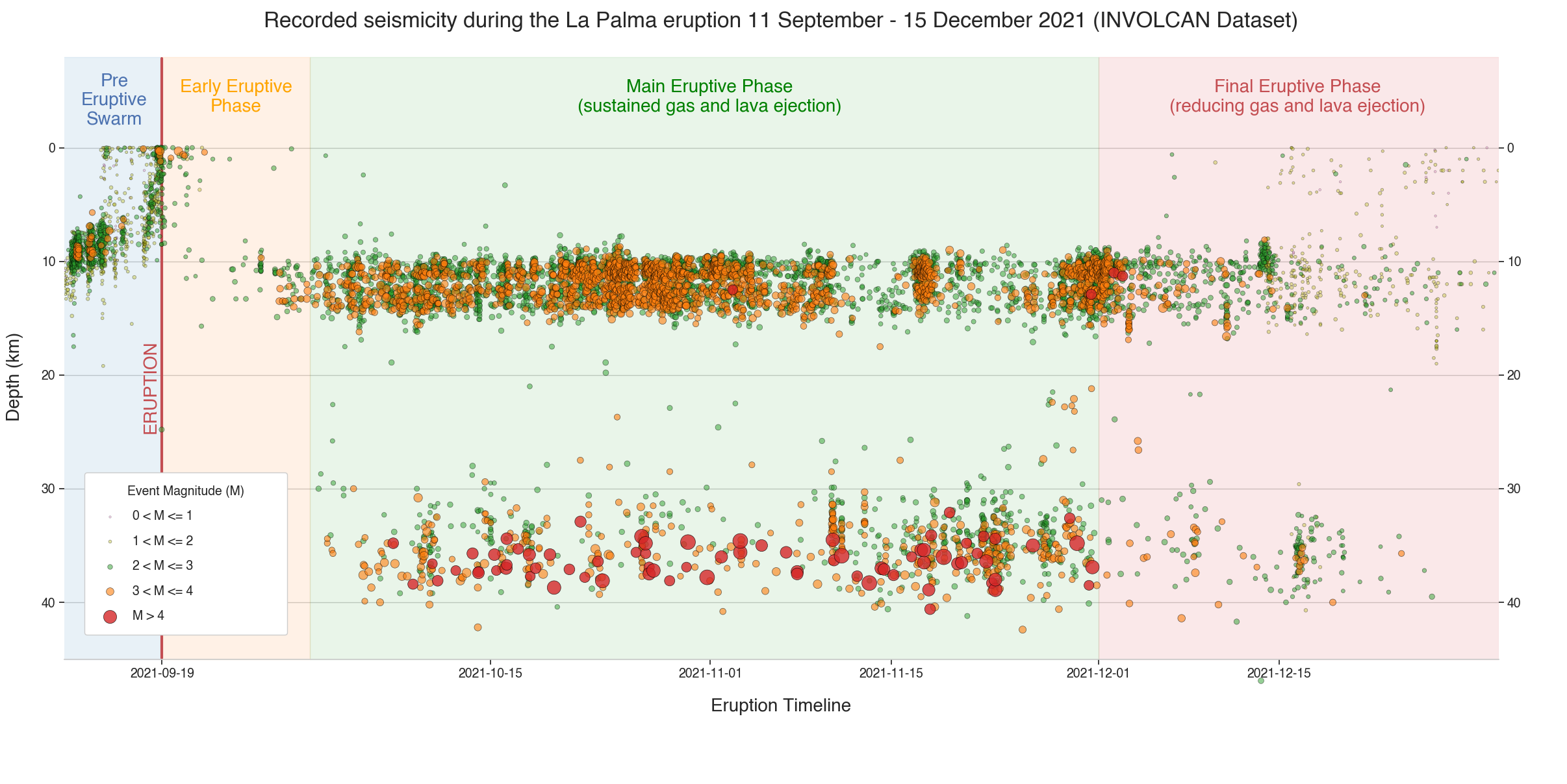

Figure 3: Earthquake data over time (n=5465) to understand their distributions spatially, by depth, by magnitude and in time.

Cumulative Distribution Plots

In [8]:

def cumulative_events_mag_depth(df, hue='Depth', kind='scatter', ax=None, dpi=100, palette=None, kde=True):
    matplotlib.rcParams['ytick.labelright'] = False
    g = sns.jointplot(x="Magnitude", y="Depth(km)", data=df,
                      kind=kind, hue=hue, height=10, space=0.1, marginal_ticks=False, ratio=8, alpha=0.6,
                      hue_order=['Shallow (<18km)', 'Interchange (18km>x>28km)', 'Deep (>28km)'],
                      ax=ax, palette=palette, ylim=(-2,50), xlim=(0.3,5.6), edgecolor=".2", marginal_kws=dict(bins=20, hist_kws={'edgecolor': 'black'}))
    if kde:
        g.plot_joint(sns.kdeplot, color="b", zorder=1, levels=15, ax=ax)
    g.fig.axes[0].invert_yaxis();
    g.fig.set_dpi(dpi)

In [9]:

import warnings

with warnings.catch_warnings():
    warnings.simplefilter("ignore")
    cumulative_events_mag_depth(df_ign, hue=None, dpi=200)
    plt.suptitle('Cumulative Events 01-01-2017 to 01-01-2022', y=1.01);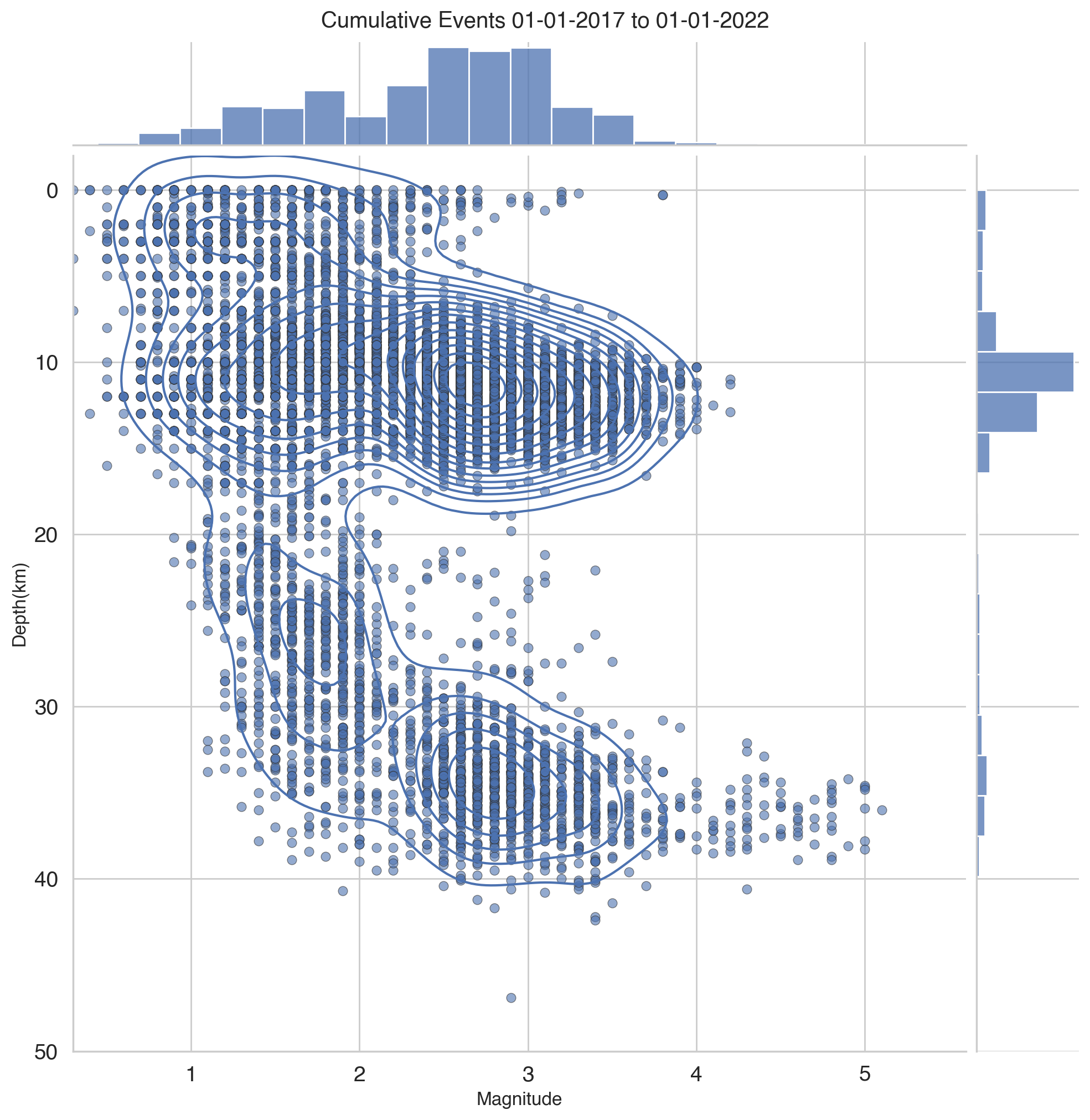

Figure 4: Cumulative earthquake data over time (n=5465) to understand their distributions spatially, by depth and magnitude.

Results

The dataset was loaded into this Jupyter notebook and filtered down to La Palma events only. This results in 5465 data points which we then visualized to understand their distributions spatially, by depth, by magnitude and in time.

From our analysis above, we can see 3 different systems in play.

Firstly, the shallow earthquake swarm leading up to the eruption on 19th September, related to significant surface deformation and shallow magma intrusion.

After the eruption, continuous shallow seismicity started at 10-15km corresponding to magma movement in the crustal reservoir.

Subsequently, high magnitude events begin occurring at 30-40km depths corresponding to changes in the mantle reservoir. These are also continuous but occur with a lower frequency than in the crustal reservoir.

Conclusions

From the analysis of the earthquake data collected and published by IGN for the period of 11 September through to 9 November 2021. Visualization of the earthquake events at different depths appears to confirm the presence of both mantle and crustal reservoirs as proposed by Marrero et al. (2019).

Availability

A web scraping script was developed to pull data into a machine-readable form for analysis. That code tool is available on GitHub along with a copy of recently updated data.

References

Marrero, José, Alicia García, Manuel Berrocoso, Ángeles Llinares, Antonio Rodríguez-Losada, and R. Ortiz. 2019. “Strategies for the Development of Volcanic Hazard Maps in Monogenetic Volcanic Fields: The Example of La Palma (Canary Islands).” Journal of Applied Volcanology 8 (July). https://doi.org/10.1186/s13617-019-0085-5.